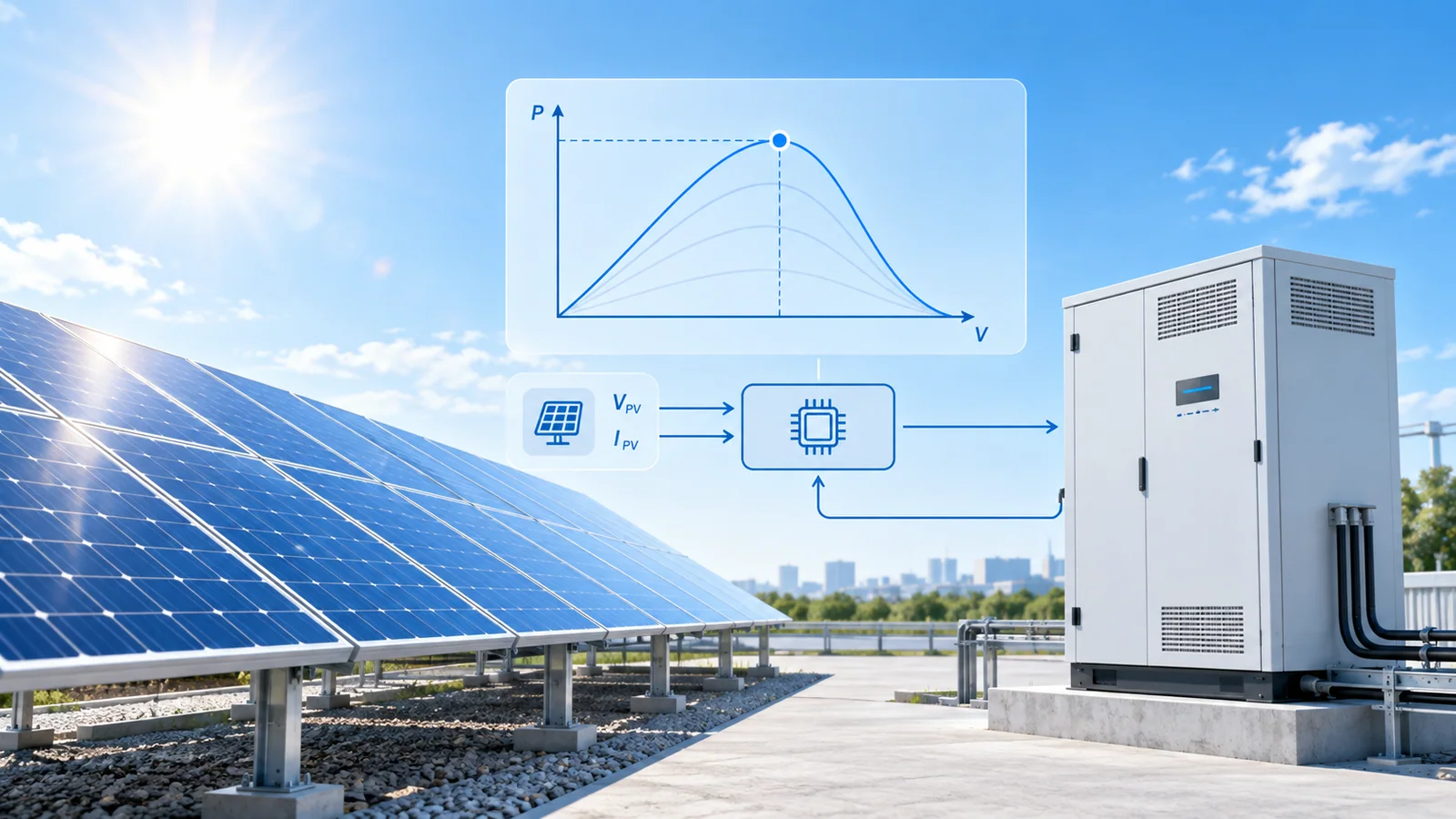
MPPT Algorithms for PV Systems: Methods Compared

A maximum power point tracking (MPPT) algorithm controls the electrical operating point of a photovoltaic array so the connected converter can extract as much available DC power as practical. It repeatedly measures or estimates voltage and current, changes a converter or inverter command, and determines whether the new operating point moved toward or away from the maximum of the array’s power-voltage curve.

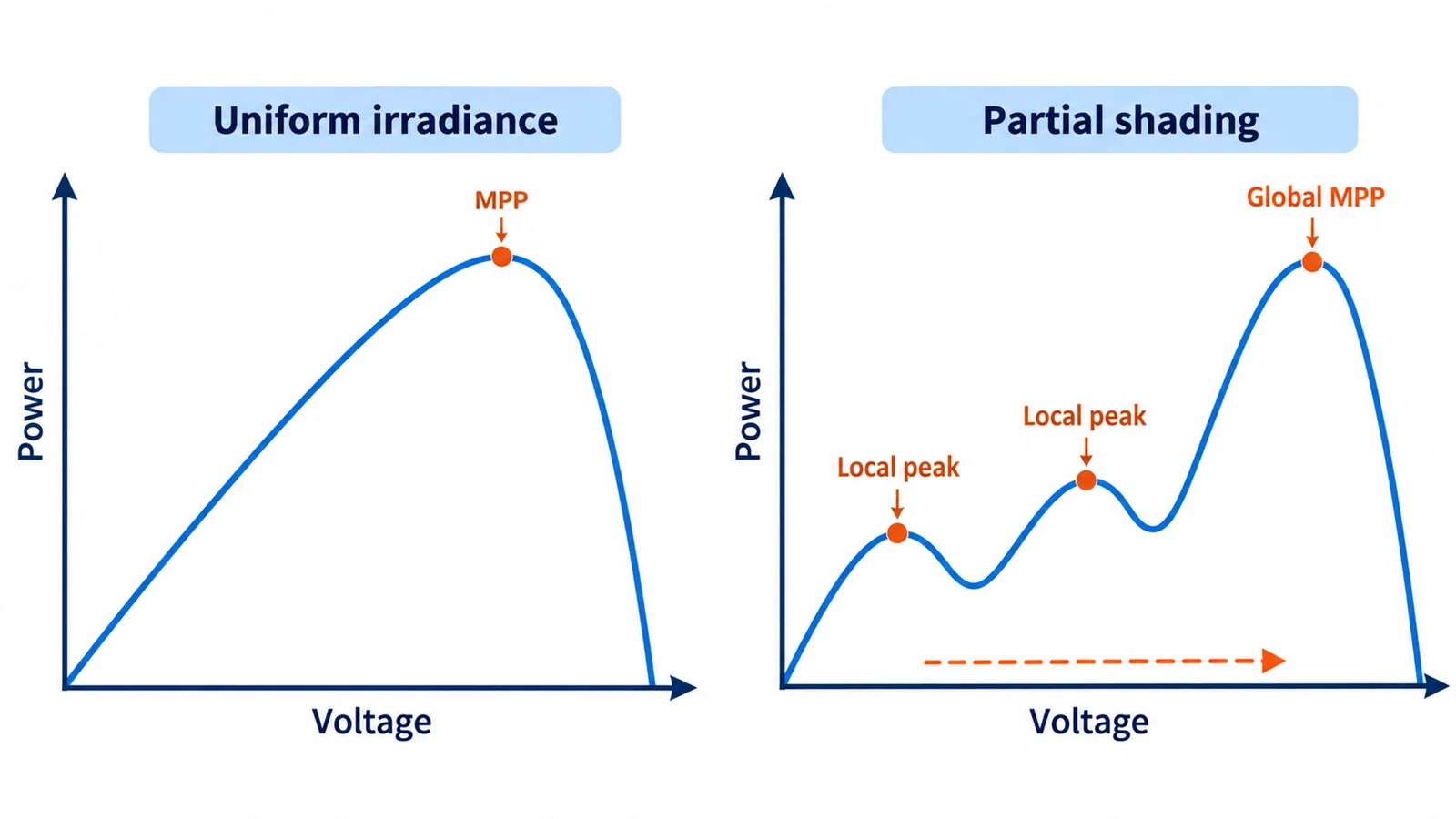
No algorithm is best for every PV system. Perturb and observe is simple and widely applicable but normally oscillates around the operating point and can move in the wrong direction during rapid irradiance changes. Incremental conductance uses the slope of the power curve and can distinguish some environmental changes more effectively, but it requires more calculation and dependable measurements. Under partial shading, the curve can contain several local peaks, so a local tracker may need a periodic or event-driven global search.

The electrical problem MPPT solves

For any operating point:

P = V × I

PV current and voltage are not independent. Their relationship changes with irradiance, cell temperature, spectral conditions, mismatch, shading and the array configuration. At short circuit, voltage is near zero, so power is near zero. At open circuit, current is near zero, so power is again near zero. Between those limits is at least one operating point where voltage multiplied by current is greatest.

The inverter or DC-DC converter presents an effective load to the array. By adjusting duty cycle, DC-link control or another internal command, it changes array voltage and current. The MPPT logic observes the result and updates the command. It does not physically move the modules and cannot create energy unavailable from the array; it seeks a better electrical operating point for the conditions that exist.

PV power-voltage curves showing one maximum under uniform irradiance and multiple local peaks under partial shading — Uniform conditions often produce one dominant power maximum, while partial shading and bypass-diode operation can create several local maxima.

Why the maximum power point moves

The maximum is not a fixed percentage of nameplate voltage. Important influences include:

Irradiance: array current changes strongly with available sunlight, and the optimum point shifts.
Cell temperature: higher cell temperature usually reduces module voltage and moves the optimum voltage.
Shading and mismatch: unequal current among modules or strings can activate bypass paths and reshape the curve.
Soiling and degradation: nonuniform losses can alter both available power and curve shape.
Electrical architecture: string length, parallel strings, optimizers and multiple inverter trackers determine which modules share one operating point.
Converter constraints: minimum and maximum input voltage, current limits, power limits and DC-link requirements can prevent operation at the array’s theoretical maximum.

Sandia’s PV Performance Modeling Collaborative explains that an array I-V curve is formed from the constituent module and string behavior. Its array-utilization guidance also separates array maximum power from the operating power actually used by the inverter, which is important when clipping or input limits apply.

The control loop in plain language

Most practical trackers repeat a sequence:

Sample array voltage and current.
Calculate power or a slope-related quantity.
Compare the sample with one or more previous samples.
Change the voltage reference, current reference or converter command.
Allow the power stage and measurements to settle.
Decide whether to continue, reverse, reduce the step or initiate another search.

Sampling interval and perturbation size are design variables. Large, frequent steps can find a moving maximum quickly but increase steady-state power ripple. Small, slow steps reduce ripple but may lag fast cloud edges or temperature changes. Measurement noise, converter dynamics and digital resolution set practical limits; an algorithm cannot make reliable fine decisions from unstable data.

Perturb and observe

Perturb and observe (P&O), sometimes called hill climbing in a broader sense, changes the operating command by a small amount and observes the resulting power:

if power increases, it continues in the same direction;
if power decreases, it reverses direction.

Near the maximum, repeated perturbations normally move the operating point from one side of the peak to the other. This creates a tracking loss that depends on step size, timing and filtering. Adaptive-step versions use larger changes when far from the apparent maximum and smaller changes nearby.

P&O strengths

Simple logic and modest processing demand.
Does not require detailed module parameters.
Practical for many single-peak operating conditions.
Easy to combine with adaptive steps and operating limits.

P&O limitations

It must perturb to observe, so some steady-state oscillation is inherent.
A rapid irradiance change can change power during the observation interval. The controller may attribute that change to its own perturbation and move in the wrong direction.
Basic P&O is a local search. On a multi-peak curve it may settle at a local maximum.
Poorly chosen timing can interact with converter transients or noisy sensors.

An IEEE comparison of P&O and incremental-conductance approaches discusses tradeoffs under different dynamic conditions. Later work continues to refine drift detection and step selection, illustrating that the implementation details matter as much as the family name; one example is this IEEE paper on improved P&O behavior.

Incremental conductance

Incremental conductance begins with the derivative of power:

dP/dV = I + V(dI/dV)

At the maximum of a smooth, single-peak P-V curve:

dP/dV = 0, therefore dI/dV = -I/V

To one side of the maximum the slope is positive; to the other side it is negative. The controller estimates incremental changes in current and voltage and compares them with instantaneous conductance. It then moves the reference toward the point where the estimated slope is zero.

Incremental-conductance strengths

Uses an explicit estimate of the power-curve slope.
Can hold the command when the maximum condition is judged to be met rather than perturbing continuously in an idealized implementation.
Can better distinguish some rapid irradiance changes from controller-induced changes when measurements and logic are well designed.

Incremental-conductance limitations

Sensitive to small differences between sampled values, so noise and quantization can destabilize the decision.
Requires thresholds for the practical meaning of “zero” slope.
More calculation and tuning are needed than for basic P&O.
It remains a local method unless extended with a global-search mechanism.

Fractional and model-based methods

Fractional open-circuit voltage assumes the optimum array voltage is approximately related to open-circuit voltage. Fractional short-circuit current applies a similar relationship to current. These methods can be inexpensive and fast, but the fraction varies with module technology and operating conditions. Directly measuring open-circuit voltage or short-circuit current can also interrupt normal production unless a pilot cell or estimation method is used.

Model-based trackers estimate the optimum from temperature, irradiance or an electrical model. They may reduce searching when the model and sensors are accurate, but parameter error, aging and mismatch can offset the benefit. Hybrid controllers often use a model or fractional estimate to reach the neighborhood of the maximum, then use P&O or incremental conductance for local refinement.

Partial shading and global MPPT

Under uniform irradiance, an array commonly presents one dominant maximum. With partial shading, bypass diodes and series-connected modules can produce steps in the I-V curve and multiple peaks in the P-V curve. A local tracker can stop at the first peak it encounters even when another peak has higher power.

Global MPPT methods address this by exploring a wider voltage range. Common strategies include:

periodic voltage sweeps;
scans triggered by a power change or mismatch indicator;
partitioning the allowable voltage range and comparing candidate regions;
hybrid global search followed by a fast local tracker;
model-assisted estimates based on likely bypass-diode states.

Searching has a cost. While the controller explores, it may move away from the current best point, and a full sweep may disturb the DC bus. Search frequency should therefore reflect how often shading patterns change, the energy at stake and the converter’s operating constraints. Complex optimization methods can be useful, but labels such as neural, fuzzy, swarm or evolutionary do not by themselves prove higher field energy yield.

The IEA PVPS and Sandia report on partial shading provides broader context on shade mechanisms, mismatch and mitigation. Good array layout remains the first control: an algorithm cannot fully recover irradiance blocked by an obstacle.

Method comparison

Method family	Measurements or inputs	Main advantage	Main limitation	Typical fit
Fixed voltage	Voltage	Very simple	Does not follow changing conditions accurately	Narrow, predictable applications rather than general energy harvesting
Fractional voltage/current	Voltage or current plus a reference relationship	Fast estimate with low computation	Relationship varies and reference measurement may interrupt operation	Low-cost control or initial estimate
Perturb and observe	Usually voltage and current	Simple and robust under many single-peak conditions	Oscillation, dynamic drift and local-peak risk	General-purpose local tracking
Incremental conductance	Voltage and current with incremental calculation	Direct slope decision and potentially better dynamic behavior	Noise sensitivity and tuning complexity	Faster-changing conditions with adequate sensing
Global scan plus local tracker	Voltage and current over a wider search range	Can escape local maxima	Search time and temporary energy loss	Arrays with material, changing partial shade
Model-based or hybrid	Electrical measurements plus parameters and possibly environmental sensors	Can initialize or predict the optimum quickly	Model and sensor errors	Systems that can support calibration and validation

Selecting an MPPT approach

Use the operating environment and converter architecture rather than algorithm popularity:

Define the curve shape. Is the tracker expected to see one peak, or can strings under its control experience nonuniform shade and multiple peaks?
Define dynamics. How quickly do irradiance, shade and temperature change relative to the electrical and control time constants?
Map converter limits. Confirm the array’s expected MPP voltage remains within the MPPT window and below current and power limits across temperature extremes.
Quantify sensing quality. Check sensor accuracy, bandwidth, sampling alignment, filtering and calibration.
Set the objective. Maximum instantaneous power, daily energy, stable DC-link operation, low ripple and component stress are related but not identical objectives.
Plan abnormal states. Startup, shutdown, clipping, curtailment, anti-islanding, low irradiance and faults may intentionally override MPPT.
Validate with representative profiles. Test steady irradiance, ramps, cloud transients, temperature variation and realistic shade patterns.

Multiple independent trackers can reduce mismatch by allowing groups of strings to operate at different voltages. Module-level power electronics can make the control boundary smaller still, but they add components, conversion stages and monitoring considerations. Architecture should be evaluated through lifecycle energy, reliability, safety and maintenance—not MPPT efficiency alone.

Measuring MPPT performance

MPPT efficiency compares energy or power captured by the tracker with the maximum available under a defined test condition. It is different from converter efficiency:

MPPT efficiency reflects how closely the controller follows the available maximum.
Conversion efficiency reflects losses while converting DC power.
Overall energy conversion is affected by both, plus clipping, standby consumption, wiring losses, thermal limits and downtime.

IEC 62891:2020 defines procedures for measuring static and dynamic MPPT efficiency of grid-connected PV inverters. Static testing examines stable operating conditions, while dynamic testing uses changing characteristics intended to represent moving maximum-power conditions. A single headline efficiency cannot describe every array curve, irradiance profile or shade pattern, so test conditions must accompany the result.

During commissioning or troubleshooting, record array voltage, current, DC power, irradiance where available, cell or backsheet temperature, tracker state, converter limits and AC output. A low operating voltage is not automatically an MPPT failure; it may reflect clipping, curtailment, startup thresholds, a DC fault, string mismatch or a deliberate protection state.

Common implementation mistakes

Treating module voltage at standard test conditions as a fixed operating voltage.
Ignoring cold-weather open-circuit voltage and hot-weather MPP voltage when checking the inverter window.
Sampling voltage and current at different instants during rapid transients.
Increasing perturbation frequency without allowing the power stage to settle.
Claiming global tracking while testing only a single-peak curve.
Confusing inverter conversion efficiency with tracking efficiency.
Evaluating shade algorithms without including the energy cost of scans.
Using one tracker for strings with materially different orientations or shade profiles without an energy study.
Diagnosing every production shortfall as an MPPT problem before checking soiling, outages, clipping and sensor quality.

Bottom line

MPPT is a closed-loop operating-point problem. P&O offers simple local tracking, incremental conductance estimates the slope more explicitly, and global-search extensions become important when partial shading creates several candidate peaks. The right design depends on curve shape, environmental dynamics, sensing quality, converter limits and the cost of searching. Compare algorithms with defined static and dynamic tests, then validate them against the real array architecture and operating profiles.

MPPT Algorithms in PV Systems: How They Work and Compare