Short answer
Kirchhoff’s current law (KCL) says that the currents entering and leaving a circuit node must balance. Kirchhoff’s voltage law (KVL) says that the voltage rises and drops around a closed loop must balance. Together with Ohm’s law, these two conservation statements let you write equations for circuits that cannot be reduced to a simple series or parallel combination.
KCL is a charge-balance rule: charge should not accumulate without limit at a normal circuit node. KVL is an energy-balance rule for a closed loop under the lumped-circuit model. The hard part is not memorizing sum of currents equals zero or sum of voltages equals zero; it is assigning reference directions, applying signs consistently and checking the answer.
The vocabulary needed before writing equations
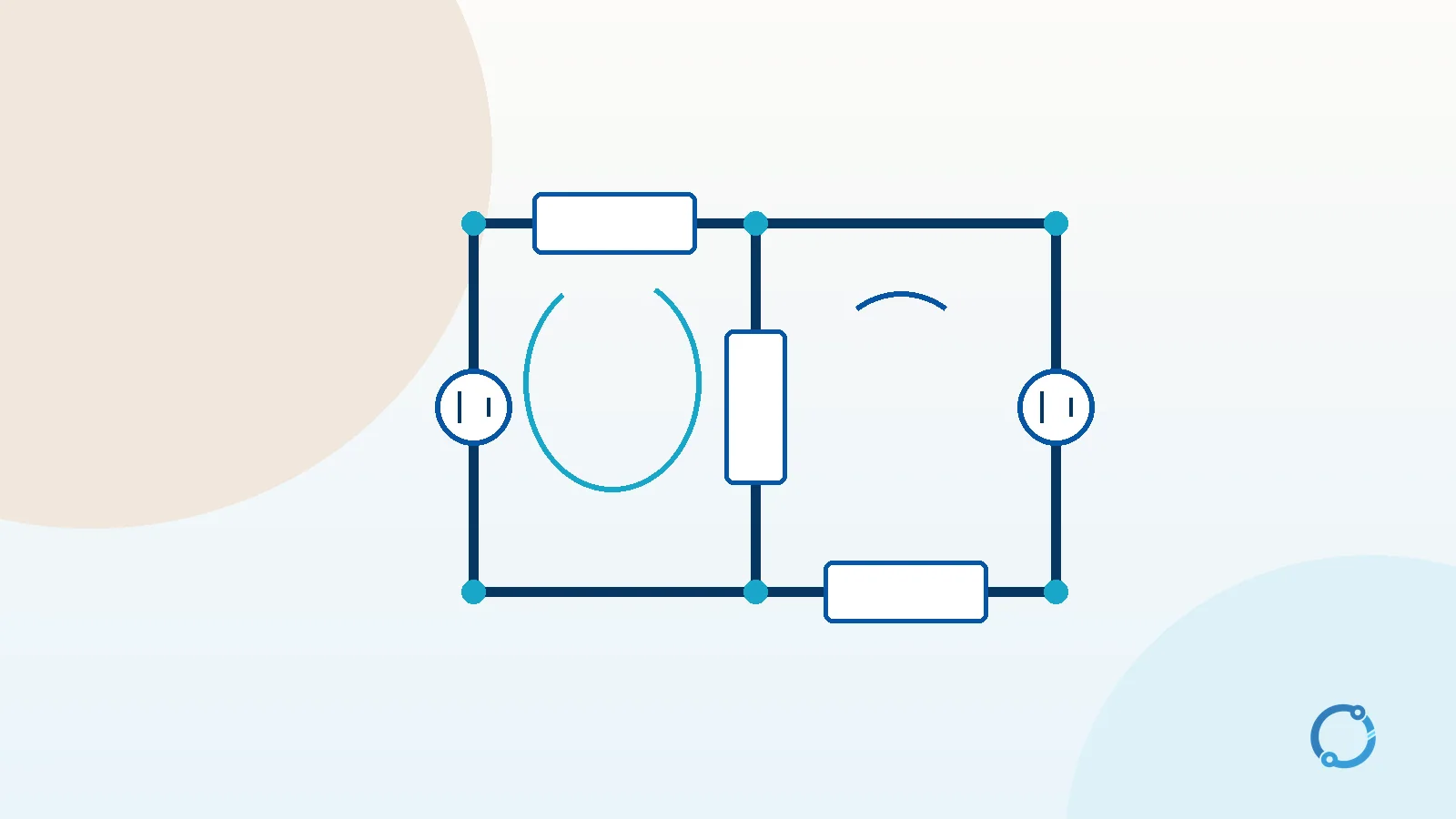
A node is a point where two or more circuit elements meet. A branch is a path between two nodes and carries a defined current in the model. A loop is any closed path through a circuit. A mesh is a simple loop that does not contain another loop inside it.
A reference direction is an assumed arrow for a current or voltage. It does not have to match the eventual physical direction. If the solved value is positive, the physical direction agrees with the arrow. If it is negative, the physical direction is opposite the arrow. A negative result is not an error; it is evidence that the initial assumption was reversed.
This convention is especially important in multi-source circuits. Two sources can push current through the same branch in opposite directions, so the direction may not be obvious before solving. Choose a direction, mark it clearly and keep the sign convention for every equation.
Kirchhoff’s current law
KCL states that the algebraic sum of currents at a node is zero when entering and leaving currents are given opposite signs:
sum I_node = 0
Equivalently, the total current entering a node equals the total current leaving it. The physical reason is charge conservation. In a lumped circuit model, charge does not pile up at an ideal node indefinitely; the current arriving must be balanced by current leaving.
Consider a node with 5 A and 3 A entering. One known branch carries 4 A away. If the unknown branch also leaves the node, then:
5 A + 3 A = 4 A + I_unknown
I_unknown = 8 A - 4 A = 4 A
The unknown branch carries 4 A in the assumed leaving direction. The check is simple: 5 A + 3 A = 8 A enters and 4 A + 4 A = 8 A leaves.
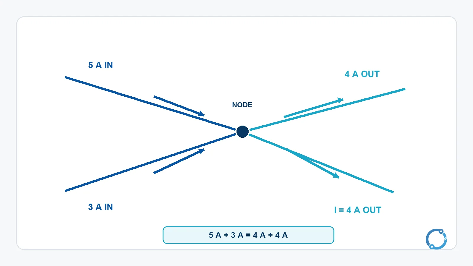
KCL is not restricted to a single wire or a simple junction. At a node connecting several branches, write every current using the same sign convention. A current entering can be positive and a current leaving negative, or the opposite convention can be used, provided that it is applied consistently.
A useful way to check a KCL equation is to return to the physical picture. If three paths meet at a junction and two carry current toward it, the third must carry the combined current away, unless another unlisted connection exists. A missing branch, a misplaced arrow or a sign reversal will make the balance fail. This is why KCL is often the quickest check on a result obtained from mesh analysis.
The rule also applies when the branch currents are changing with time. At each instant, the algebraic sum of the currents at an ideal lumped node remains zero. In a real conductor, charge can redistribute and a small amount of charge can be stored in stray capacitance, but the lumped model treats that storage as an explicit element rather than hiding it inside the node.
Kirchhoff’s voltage law
KVL states that the algebraic sum of voltage changes around a closed loop is zero:
sum V_loop = 0
Equivalently, the total voltage rise around a loop equals the total voltage drop. In the lumped-circuit model, moving around a closed path returns to the same potential, so the changes must cancel.
KVL requires a sign convention. For this article:
- Moving through a source from its negative terminal to its positive terminal is treated as a rise.
- Moving through a source from positive to negative is treated as a drop.
- Moving through a resistor in the direction of the assumed current produces a voltage drop.
- Moving through a resistor opposite to the assumed current produces a voltage rise.
These rules are a bookkeeping system, not a claim that every source or resistor always has one fixed polarity. The chosen arrows and the signs in the equations must travel together.
A second useful check is to reverse the direction of traversal. If a loop is traced in the opposite direction, every signed term should change sign, but the equation should still be true. If the result changes in a way that cannot be explained by that sign reversal, the original equation probably mixed two conventions. Good circuit notation is therefore not cosmetic: arrows and labels are part of the mathematical model.
A single-loop voltage check
Take a 12 V source connected to a 4 ohm resistor and an 8 ohm resistor in series. The total resistance is:
R_total = 4 ohm + 8 ohm = 12 ohm
The current is:
I = V / R_total = 12 V / 12 ohm = 1 A
The resistor drops are:
V_4 = I x 4 ohm = 1 A x 4 ohm = 4 V
V_8 = I x 8 ohm = 1 A x 8 ohm = 8 V
Around the loop, the source rise is 12 V and the two drops sum to:
4 V + 8 V = 12 V
The rise and drop balance. This is the same result obtained by the series rules in the series and parallel circuits guide, but KVL shows why the resistor voltages add to the source voltage.
This simple case also demonstrates that a KVL equation is not a separate replacement for Ohm’s law. The voltage across each resistor is unknown until the current is known, and Ohm’s law supplies that relationship. KVL supplies the connection statement that the two resistor drops must account for the source rise. Combining the connection equation with the element equations produces a solvable system.
The Ohm’s law guide supplies the relationship used inside each resistor. KVL does not replace Ohm’s law; it connects the element voltages around a loop. The voltage article explains the potential-difference interpretation behind each signed voltage change.
A two-loop worked example
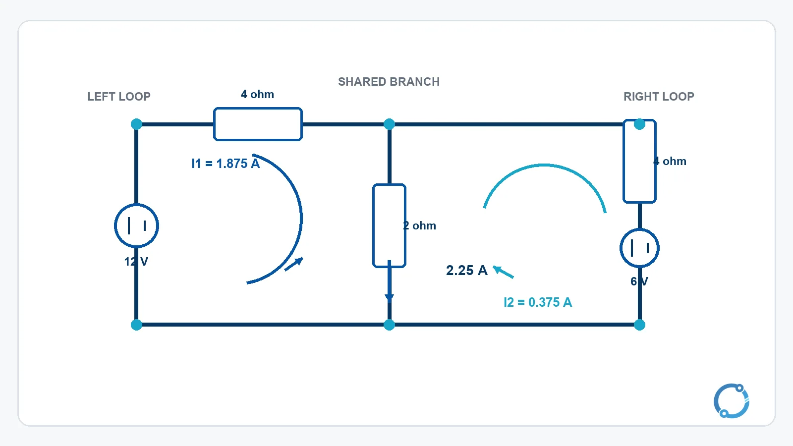
The real value of Kirchhoff’s laws appears when a circuit has more than one loop. Consider a left loop with a 12 V source and a 4 ohm branch, a right loop with a 6 V source and a 4 ohm branch, and a shared middle branch of 2 ohm.
To keep the shared-branch contributions easy to track, define the loop-current reference arrows so that both I1 and I2 pass downward through the 2 ohm branch. The left loop current I1 follows a clockwise path. The right loop current I2 follows a counterclockwise path. These are reference choices; if either solved value is negative, the actual current is opposite the arrow.
For the left loop, the 4 ohm branch and the shared 2 ohm branch carry I1 and I1 + I2 respectively:
4 I1 + 2(I1 + I2) = 12
6 I1 + 2 I2 = 12
For the right loop, the own 4 ohm branch carries I2 and the shared branch again carries the sum:
4 I2 + 2(I1 + I2) = 6
2 I1 + 6 I2 = 6
We now have two equations in two unknowns:
6 I1 + 2 I2 = 12
2 I1 + 6 I2 = 6
Multiply the second equation by 3:
6 I1 + 18 I2 = 18
Subtract the first equation from this result:
(6 I1 + 18 I2) - (6 I1 + 2 I2) = 18 - 12
16 I2 = 6
I2 = 6 / 16 = 0.375 A
Substitute I2 into the first equation:
6 I1 + 2 x 0.375 = 12
6 I1 + 0.75 = 12
6 I1 = 11.25
I1 = 1.875 A
The shared branch current is the sum of the two chosen loop currents:
I_shared = I1 + I2 = 1.875 A + 0.375 A = 2.25 A
The result is fully consistent with the assumed arrows. The left loop sends 1.875 A downward through the middle branch, the right loop sends 0.375 A in the same reference direction, and the branch total is 2.25 A.
The algebra can be checked by substituting both values into the second loop equation:
2 x 1.875 A + 6 x 0.375 A
3.75 A + 2.25 A = 6 A
The equation also balances. The two source equations are therefore mutually consistent. If one equation balanced and the other did not, the next step would be to check the signs, the loop direction and the shared-branch term before changing any numerical value.
Verify the result with KCL
The solution can be checked without assuming that the mesh equations are correct. At the shared node, the two left and right contributions join in the reference direction used in the diagram. The shared branch current is the sum:
1.875 A + 0.375 A = 2.25 A
This matches the branch current calculated from the loop equations. The check is valuable because a sign error often produces two plausible individual numbers that fail at the shared branch. KCL turns the node into an independent consistency test.
The electric current article explains how to interpret the resulting current direction, including what a negative answer means when the assumed arrow points the other way. The sign is part of the model, not a reason to discard the solution.
A four-step method
For a linear DC circuit, a reliable workflow is:
- Draw and label every node, branch, source and resistor.
- Assign reference directions to all unknown currents and mark the polarity of every voltage.
- Write KCL at the nodes needed to relate currents and KVL around the meshes or loops needed to relate voltages.
- Solve the simultaneous equations, then check the answer with KCL, KVL or a power balance where appropriate.
The number of independent equations must match the number of unknown currents or voltages. In this article’s two-loop example, there are two unknown loop currents and two independent loop equations. If a circuit has more nodes and branches, the same method can produce a larger system; a computer or linear-algebra tool is then useful for bookkeeping.
It is also useful to distinguish a mathematical solution from a physically reasonable one. A very large current may indicate a missing resistance, an incorrect source value or a branch that should not be treated as ideal. After solving, check the magnitudes, the units and the expected direction of energy flow. The equation can be algebraically correct while the circuit model is incomplete.
When series and parallel rules are enough
Do not use a full nodal or mesh analysis when a simple series-parallel reduction already solves the problem. The series and parallel circuits guide explains how to combine resistors when the current paths are straightforward. That is faster and less error-prone for a simple network.
Kirchhoff’s laws become essential when sources are distributed, when a bridge or multi-loop network cannot be reduced to one series path and one parallel group, or when a shared branch makes the current depend on more than one source. The circuit’s topology should choose the method, not the other way around.
For hand analysis, mesh currents are often convenient when the circuit has several obvious windows. Nodal analysis is often convenient when the unknown voltages are the main quantities of interest. Both approaches use KCL and KVL, but they package the equations differently. The choice is a workflow decision, not a different physical law.
KCL and KVL also provide the foundation for computer circuit simulation. A simulator builds a large system of equations from the connections and element models, then solves it numerically. The labels and algorithms differ from a hand calculation, but the conservation rules remain the underlying structure.
Applicability boundaries
KVL and KCL are normally introduced for lumped circuits, where the physical dimensions are small enough compared with the relevant wavelength that a node can be treated as having one potential and a wire can be treated as a connection. At low frequency, this model works well for many power and electronic circuits.
KVL has another boundary when a changing magnetic flux links the loop. In that case, the electric field is not conservative in the simple lumped sense, and the voltage around the physical contour must account for the induced electromotive force. A transformer core, a wire loop near a switching magnetic field or a high-frequency layout can make the simple scalar-voltage model insufficient. The article does not attempt to replace an electromagnetic field analysis; it identifies where the beginner’s KVL model stops being enough.
The laws also depend on consistent component models. A resistor is not perfectly constant, a source may have internal impedance and a wire may have resistance or inductance. Kirchhoff’s laws still express the connection constraints, but the element equations must represent the actual components. The power-factor guide is a reminder that AC circuits can include phase-shifting energy storage, so a DC-only mental model is not enough for every network.
Frequently asked questions
What is Kirchhoff’s current law in simple terms?
At a node, the current entering must equal the current leaving when the signs are assigned consistently. Charge does not disappear or accumulate indefinitely at an ideal lumped node.
What is Kirchhoff’s voltage law in simple terms?
Around a closed loop, the algebraic sum of voltage rises and drops is zero. Moving around the loop returns to the same potential, so the changes balance.
Why can a calculated current be negative?
A negative answer means the actual current points opposite the reference arrow you selected. The magnitude is still correct. Reverse the arrow if you want the final diagram to show the physical direction.
Do Kirchhoff’s laws work for AC circuits?
They apply to the instantaneous voltages and currents of a circuit, and phasor models can represent steady sinusoidal quantities when the assumptions are valid. The element equations and sign conventions still have to match the chosen model.
Can I solve every circuit with only KCL and KVL?
They provide the connection equations, but you also need an equation for each element, such as Ohm’s law for a resistor. Nonlinear or energy-storing elements require their own models, and distributed or strongly electromagnetic circuits can fall outside the simple lumped treatment.